A (very) simple “Network Traffic Visualization” using Network Graphs

A network visualization has nodes and edges. I like to apply it to actual IT Networks Traffic visualizations, where there are connections (edges) between two IP addresses/machines (i.e. “nodes”). Let’s try and apply that to some Netflow data…

Getting the data

After some searching (that was some time ago now), I came across secrepo.com. There I found some sample datasets that can be of interest for this Blog. (Yes, one could set up a lab full of VMs, sniff some data and create a useful Netflow dataset, but this blog I work on essentially on my spare time, and I haven’t yet taken the time to set a real “lab” for now; that might come later, who knows.)

So I will use NetFlow data for this exercise. See references below to get a pointer to the dataset (careful, 500+ MB while zipped, about 2.6 GB if/when unzipped).

Part I: Playing with the data

So one thing happened here, I usually limit the RAM available to my “RStudio Server” Container (and my host memory is not unlimited). You might remember I do not use a “normal” install of RStudio (see here for more information on my setup).

Also, it gives me a chance to point to something specific about working with the R interpreter: R works “in RAM” (to summarize). Now I know there are packages out there to try and overcome these limitations, but let’s accept that limitation here for the sake of this exercise.

Whatever the case, in this instance I decide to allocate more memory to my Container before going any further.

$ docker run -it -m 2000M -v /<somepath>/:/mnt/R/ -p 8787:8787 rserver1:2.1

This is one of those cases where some basics of Linux shell come in handy: So I have a 2.6GB file, full of Netflow data in text format. I can tell what the data looks like without actually opening the 2.6GB file altogether, using:

$ head conn.log

On a Linux Shell. As the RStudio Server container I use is actually an Ubuntu container, I have access to such a shell, so that’s covered.

Next up, and for this exercise, but with value for other analysis endeavours, let’s actually “split” this big file in smaller chunks, which we will be able to read into R. Also, in this case, I don’t really want/need to actually use all the 2.6GB worth of Netflows. That’s a different exercise. So I will “sample” the data, instead.

Two Linux shell command lines will be useful there:

$ split --verbose -l100000 conn.log conn_extract_log.

This will create several files named “conn_extract_log.xx”, where “xx” starts at “aa”, and goes up. I use the “–verbose” option to see where I am at, and stop the command from going on manually with “Ctrl-C”.

That way, I have a few manageable files of 100000 lines extracted from the beginning of the original file. But then, I wanted a “sample”, ideally something random, from such extracts. Once again, one can use a Shell command as such:

$ sort -R conn_extract_log.aa | head -n1000

You get the idea, I’ll have to go across a few of the extracts to sample a subset of random lines, which in turn will be a sample of 1000 lines out of the few initial hundreds of thousands.

Obviously, this is far from perfect: it would have been better to go random across the original 2.6GB file, for instance, and then split or head a few thousands. Better even, extract a few hundred thousand lines and then go sampling random entries. But once again this is an exercise and I mean to explain the process, not just “do it”.

So yes, ideally, you could go the other way around, and all the above can be achieved better with something like:

$ head -n500000 conn.log | sort -R | head -n 10000 > second_sample.log

OK, so now we have a manageable dataset for the exercise.

IMPORTANT NOTE: “Sampling” is not a process to be taken lightly. The above (taking 10000 entries out of the first 500 thousand) was completely arbitrary and MIGHT NOT be the correct way to go in a real world exercise. The above was just an exercise to demonstrate a few ways of how one COULD extract a few lines from a big file to work with a more manageable dataset (i.e. smaller, in this case). Please see a future post on sampling if you need to do it in a real world setting.

Part II: What’s next?

Well, for now, I basically have NO IDEA what the dataset I will be using looks like.

I should do (in a real world exercise) some “Exploratory Data Analysis”. But this entry will not cover all of a real world exercise (for instance, we’d separate private from public IP address, distinguish IPv6, identify the distribution of the connections (numbers, per pair, or with volumes of data transferred), the types (web, etc. using the port), and a potentially long list of more details that we could want to understand.

Allow me to skip to the Network Graph, as I have a grasp on what a Netflow entry provides…

In order to do so, I like the package “visNetwork”, available as a CRAN package.

Preparing the data

Let’s try to visualize the connections between pairs of IP addresses. This should be straight forward, as the NetFlow informs about such connections.

For this exercise, we will create a very simple version, nothing “fancy”, just nodes (IP addresses) and links between them (connections), with no further enhancements (modifying sizes by number of connections, colouring connections by port number, etc.).

Tip: You can in theory generalize and use the code below to create “network graphs” from any two character columns in any data.frame.

So we are going to need to create two datasets:

The list of connections, from one IP address to another.
The list of “nodes”, each node being an IP address.

Moreover, visNetwork expects identifiers of nodes for the list of connections, rather than names of nodes.

We should first read the data into our R environment:

conns <- read.csv("/mnt/R/Demos/conn_extracts_log/second_sample.log", header = FALSE, sep = "\t")

Then we will keep only the pairs of IP addresses:

conns_from_to <- conns[, c("V3", "V5")]
names(conns_from_to) <- c("from", "to")

We won’t be using much more of the data, and some IP pairs will probably appear several times, so we use the dplyr functions “distinct()”:

conns_from_to <- conns_from_to %>% distinct()

The function read.csv (contrary to the behaviour of data.table “fread”) will cast IP addresses to factors, which we do not want here:

conns_from_to[] <- sapply(conns_from_to, as.character)

We keep, for the sake of the exercise, only IPv4. We created a function in a former post to check for IPv4 correct format:

# If we look at it, we might see IPv6 in there. Let's simplify a bit the dataset and focus on IPv4:
is_valid_ip_string_format <- function(ip = NA) {
    is.character(ip) && grepl("^((25[0-5]|2[0-4][0-9]|[01]?[0-9][0-9]?)(\\.|$)){4}", ip)
}
# Now we keep only the IPv4:
conns_from_to <- conns_from_to[sapply(conns_from_to$from, is_valid_ip_string_format) &
    sapply(conns_from_to$to, is_valid_ip_string_format), ]

Then we create the “nodes” list, with identifiers:

nodes <- unique(c(conns_from_to$from, conns_from_to$to))
conns_nodes <- data.frame(id = seq(1:length(nodes)), node = nodes)

Almost there. But we still need to change IP addresses in the connections list to identifiers. There are many ways, arguably some better, other worse. Let’s demo a couple of options here:

# OK so finally, let's merge things (one way to go, NOT optimal):
conns_from_to <- merge(conns_from_to, conns_nodes, by.x = "from", by.y = "node", all.x = TRUE)
conns_from_to <- conns_from_to[, -1]
conns_from_to$from <- conns_from_to$id
conns_from_to$id <- NULL

# Or another option (not perfect either):
conns_from_to$to <- sapply(conns_from_to$to, function(x) { conns_nodes[conns_nodes$node == x, "id"]})

OK, so we have two data.frames, and we are almost ready to “show” the connections observed in the NetFlow dataset.

The Visualization itself

Let’s add some visual parameters for the nodes:

conns_nodes$shape <- "dot" 
conns_nodes$shadow <- TRUE # Nodes will drop shadow
conns_nodes$label <- conns_nodes$node # Node label
vis.nodes$title <- conns_nodes$node # On click
conns_nodes$borderWidth <- 2 # Node border width
conns_nodes$color.background <- "lightblue"

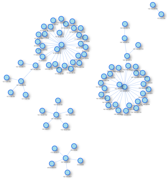
And finally, we can visualize a simplification of our dataset:

visNetwork(conns_nodes, conns_from_to)

One result (we’ve been using random selection of data to present only a subset, so results might differ):

The whole R code can be found here on my GitHub account (as usual): https://github.com/kaizen-R/R/blob/master/Sample/Visualizations/Network_graphs/Netflow_simple_visu001.R

References:

https://www.secrepo.com/Security-Data-Analysis/Lab_1/conn.log.zip