I said I would move away from the Netflows examples for a while, and so I shall. Let’s try something a bit different: Detecting Ransomware through a (very) simplistic approach.
As always, this is just an exercise, a demo of the approach one could potentially use. So some things are going to be simplified here. I’ll try to leave some pointers to a more “real-world” approach along the way, but that will be overall out of scope.
This is part one of a two-parts exercise: First, we will focus on the dataset itself.
The context
Ransomware is characterised by one thing among others: It ciphers files “massively”. Now I will not try to prevent that, but rather detect this one particular behaviour.
This should be fairly simple. We just need to look for one of two things: Sudden (and sustained) increase in files changes. Or, depending on the attack, maybe massive copy and ciphering.
Let’s assume one ransomware “gets in”, and starts ciphering files it comes across. In doing so, and unless it is more complex than in our assumption, it will update the “last edited” timestamp for each file it ciphers. That’s the “behaviour” we shall look for.
For example, on MacOSX, Linux (and the likes) one can use stat, find or ls (…):

The setup
Alright, so for the data we want to collect: We want to list, say for example every minute, all files that have been updated in the last minute, and then keep a count of the number of such files, along with the date-time of the check.
Why every minute? Well, if ever ransomware hits, one shall not wait to long to react and hence to detect something is happening…
Our goal is to end up with a VERY simple dataset: A table of two variables
- Date-time (down to the minute) on one hand
- Number of files edited in the last minute (on the other).
Clearly, nothing magical.
There are many intricacies to this though: Where to look? Do I list all files on a system?
Many files are being edited all the time, maybe in some obscure OS or application folder, while other documents (user files) might not be edited so fast, for example (or not too many at the same time).
Of course, that would also depend on whether we are looking at a user’s laptop or a server of some kind, or maybe a shared folder accessed by many users, and it might also depend on the type of user.
Because of this, “Pointer 1”: This exercise/demo (R programming) is about monitoring one folder on one system. But it could be extrapolated to many folders and/or systems rather easily. The only difference is that we would repeat the exercise in a “loop” over many such monitored resources.
And “Pointer 2”: There is obviously a matter of gathering the very simple data every minute from all resources to be monitored. I’ll leave it to each one to figure that out, but to clarify: One could use crontab and rsyslogd to send a very simple “log” to a central system gathering the data point every minute on many systems into one central folder, accessible by our R script, for example.
One could also allow our script to connect somehow (e.g. over SSH) to execute one command every minute (in turn, this assumes keys exchange (for example) between our central machine where our script runs, and all destination (Linux) boxes).
And any number of more or less complex/professional alternatives: Through Ansible, or maybe OSQuery (e.g. see this doc page of OSQuery on FIM), etc.
Whichever the solution, at the end of the day, the same script could be run to monitor several locations/machines. What will be explained about anomaly detection (expected next week) could then be applied to each source (machine).
The dataset
Let’s focus on one folder and sub-folders, on one system.
Now how do we gather our data? On a Linux-like OS, it should be accessible and plenty has been written about that, plus this is not our goal (I guess I’d go with a mix of “ls” or “stat” or “find”, “sed” and “cut”, but users of awk I am certain would do this much better). I’ll leave it to the reader, as this is beyond our scope (R Programming).
But we are interested in R here, so in our language of choice, and supposing we have read-only access to a folder of interest from our script, how do we get the number of files modified within the last minute?
# Let’s do this for the current path:
changed_last_minute <- difftime(Sys.time(),
                                file.info(list.files(path = ".", recursive = TRUE))$mtime,
                                units = "seconds") < 60
length(changed_last_minute[changed_last_minute == “TRUE"])
Just FYI, on MacOSX (I’m not too familiar with it, I usually use shell commands in Linux), I found the following command works for our goals:
find . -mmin -1 -type f -exec ls -l {} + | wc -l
Now that we know how many files have been changed in the last minute, let’s run this every minute, and save it to a data.frame:
update_last_changed_values <- function() {
  changed_last_minute <- difftime(Sys.time(),
                                  file.info(list.files(path = ".", recursive = TRUE))$mtime,
                                  units = "seconds") < 60
  data.frame(date_time = Sys.time(),
             num_changes = length(changed_last_minute[changed_last_minute == "TRUE"]))
}

changes_dataset <- update_last_changed_values()

# Simplest version and as example: Get the data for the next 5 minutes, totalling 6 rows
for(i in 1:5) {
  Sys.sleep(60)
  changes_dataset <- rbind(changes_dataset, update_last_changed_values())
}
OK so now we know how to collect the data from R. One issue of doing this, is that you need to “use” your R interpreter for this sole purpose (remember, R is interpreted and single thread). There are tricks around that, but this is out of scope for today 😉
Again, there are alternatives to gather the data, scripting, Ansible (…) for us to simply “use it”. So I will not worry about this issue here. If we really want to have one R script running to do what I want to explain next week, we could create a Dashboard in Shiny for instance, and run it from a Docker Container, looking at data centralised from several systems/folders to be monitored.
(Note: I’ll write about Shiny and Shiny dashboards soonish, hopefully.)
Dummy base dataset
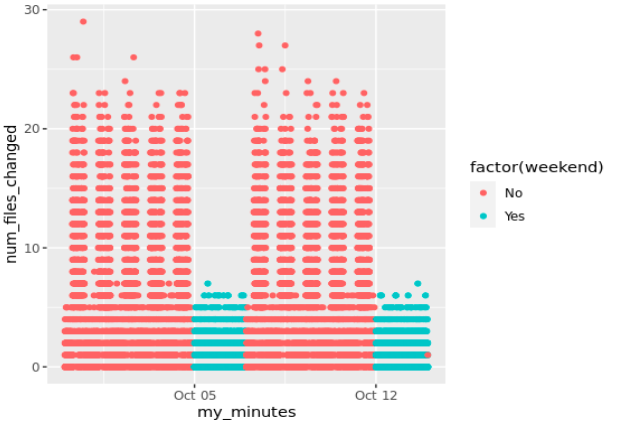
Let’s create a data.frame with all values from one week to “play with” and simulate a detection later on.
We’ll go easy: We assume “more files are opened from Monday to Friday, but for nights and lunch times; and less (next to 0) are opened on weekends”.
The following generates a VERY simplified dataset along those objectives:
# First, let's create a "dummy" dataset to play with:
# 1 week in minutes: 7 * 24 * 60
number_of_rows <- 10080

# Simulating file accesses by minutes during work day 8-18h:
workday_volumes <- function() {
day_set <- c()
for(i in 1:5) {
day_set <- c(day_set, c(round(rnorm(7*60, mean = 0, sd = 2)),
round(rnorm(6*60, mean = 10, sd = 5)),
round(rnorm(2*60, mean = 2, sd = 5)),
round(rnorm(3*60, mean = 10, sd = 5)),
round(rnorm(6*60, mean = 0, sd = 2))))
}
sapply(day_set, function(x) { ifelse(x<0, 0, round(x)) })
}

# Assuming very low volumes on weekends:
weekend_volumes <- function() {
sapply(rnorm(2*24*60, mean = 0, sd = 2), function(x) { ifelse(x<0, 0, round(x)) })

}
# Let's create our dummy dataset:

# we consider today at 00h "as a Monday":
base_time <- Sys.time()
start_date <- base_time - 3600 * hour(base_time) - 60 * minute(base_time)
start_date <- as.POSIXct(start_date, tz = "UTC")
changes_df <- data.frame(my_minutes = start_date + 60 * seq(1:number_of_rows),
num_files_changed =
c(workday_volumes(), weekend_volumes()))
# quick check
str(changes_df)
# Just for us to see it better:
weekend_rows <- (24*60*5):(24*60*7-1)
# In a real-world setup, weekends would happen on weekends... We just assumed we started
# on a Monday at 00h00.

# Let's "add features" (quotes needed, yes):
changes_df$wday <- as.POSIXlt(changes_df[,1])$wday
changes_df$hour <- as.POSIXlt(changes_df[,1])$hour
# Now what we really want is to use normal data for workdays&hours, and weekends&hours
changes_df$weekend <- "No"
changes_df[weekend_rows, "weekend"] <- "Yes"
We do that for two weeks for later use:

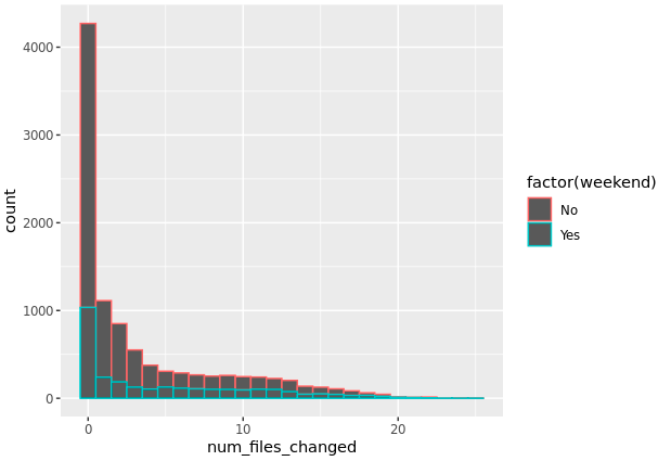
As we expect, we have lower numbers on weekends (and less weekend days):

Sure, this is VERY simplistic. Nothing near “real-life” data, way too many assumptions have been used to generate the above data. I actually have no ideas what to expect for a similar dataset in a real-world setup. Variability will be MUCH higher, and it all depends on what KIND of folder one would monitor. Or so I would expect.
But the above will have to do for the next part of the exercise. Just keep in mind, it is only a DUMMY dataset, hopefully with sufficient explanatory value.
Conclusions
In the next post, we will do the second part of this exercise, namely: injecting, and then detecting anomalies on our dataset.
(Note: I will then post to my GitHub account the associated source code)
Resources
https://osquery.readthedocs.io/en/stable/deployment/file-integrity-monitoring/