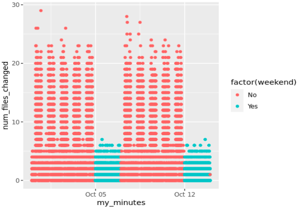
Last week, we created a “dummy” dataset of number of files edited per minute in a theoretical shared folder of users’ documents.
We did that as a setup to later demo some ways of detecting sudden changes to those numbers, expecting that would be one behaviour of a potential ransomware for us to detect.
Let’s move on to the second part now: Actually detecting an attack.
The easiest version for detection
Let’s call this the version 0 of our anomaly detection work here.
Well, the simplest way to go, is to use the max value of the number of file edits per minute as a threshold. If we assume there were no attack for data in one folder over a period of time with observations, then a “sudden increase” would be ABOVE (with our assumptions) that threshold.
So we observe data for (say) 1 week, we might consider that our “training dataset”, and take as a threshold the maximum of values observed in that time range:
anomaly_v0 <- max(changes_df[1:nrow(changes_df),2]) + 1
Very straightforward. Anything above that value (30 in my demo dataset) would signal something that is not expected.
But that value is not perfect: Over weekends, for instance, the normal value is much lower than that:

So we might want to factor that in.
Something a bit more elaborate
Now we know, from the observed above, that anything above 10 files edited per minute during weekends would be unusual. Actually, we know (because I invented the dataset) that at lunch time during workdays there is less file-edits/minute. We know there is a seasonality, by hours (this could vary).
Let’s ASSUME normality of number of files edited per minute for each hour of each day, depending on the weekday. That is, we expect to have a normal distribution of number of files edited on a Monday between 8 and 9 am. (Once again, this is true, as our dataset was generated using “rnorm” in groups of hours).
Then we can use the usual numbers of normal distributions: Anything above the mean plus 3 standard deviations would be VERY unusual, for all observed value of a Monday between 8 and 9 am. We can then do the same for each group of weekday-hour pairs. We can also assume (in our case) that edits/minute on a Monday at 9 should be similar to the same values on a Friday at 9, but very different on Sundays at 9:
changes_df_v1 <- changes_df # 1st week of data.

changes_df_v1_summaries <- changes_df_v1 %>% group_by(weekend, hour) %>%
summarize(hourly_mean = mean(num_files_changed),
hourly_sd = sd(num_files_changed))
changes_df_v1_summaries$threshold <- ceiling(changes_df_v1_summaries$hourly_mean +
3 * changes_df_v1_summaries$hourly_sd)


changes_df_v1 <- merge(changes_df_v1, changes_df_v1_summaries[,c("weekend", "hour", "threshold")],
by.x = c("weekend", "hour"),
by.y = c("weekend", "hour"),
all.x = TRUE)
changes_df_v1$alert <- "No" # default
changes_df_v1[changes_df_v1$num_files_changed > changes_df_v1$threshold, "alert"] <- "Yes"
nrow(changes_df_v1[changes_df_v1$alert == "Yes",])
Which gives us something like so, with 34 “detections” (most on the weekends) for the first week of data:

Going further: The anomalize package
Now to the “good” stuff. I recently played a bit with the “anomalize” R package. By default, this package observed timed data (like our dataset), and using time-decomposition, applies LOESS (by default) to do local regressions. Or so I have understood while reading about the package. LOESS builds on “classical” methods , such as linear and nonlinear least squares regression. This is explained better than I could do it here.
OK so, let’s test that.
# The package "anomalize" requires tibble datasets to work.
# So let's make it a tibble time object then:
dat_tibble <- as_tbl_time(changes_df, my_minutes) # 1st week of data.

# Anomalize uses time decomposition, frequency and trend. Let's use the defaults on the 1st week:
anomalize_test1 <- dat_tibble %>%
time_decompose(num_files_changed, frequency = "auto", trend = "auto") %>%
anomalize(remainder) %>%
time_recompose()

anomalize_test1 %>% plot_anomalies()

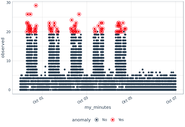
Red dots are “anomalies”. Way too many of them for our goals (765 in my tests, where we know there were no anomalies per-se by our standards). By default, “anomalize” uses certain values for frequency and trend, and defaults to Inter-Quartile Range as a detection method (so does the package forecast::tsoutliers, which is why I will not demo it here today):
> get_time_scale_template()
# A tibble: 8 x 3
  time_scale frequency trend
  <chr>      <chr>     <chr>
1 second     1 hour    12 hours
2 minute     1 day     14 days
3 hour       1 day     1 month
4 day        1 week    3 months
5 week       1 quarter 1 year
6 month      1 year    5 years
7 quarter    1 year    10 years
8 year       5 years   30 years
We do NOT want “anomalize” to use 1 day for frequency, as we know our data varies with the hours… Let’s try and adjust that:
# Now we know our frequency is about < 1 hour, and trend repeats every week.
# This is relevant data to apply LOESS
# Let's try different values, more adjusted to what we'd expect:
anomalize_test1 <- dat_tibble %>%
time_decompose(num_files_changed, frequency = "1 hour", trend = "1 week") %>%
anomalize(remainder) %>%
time_recompose()

anomalize_test1 %>% plot_anomalies()
nrow(anomalize_test1[anomalize_test1$anomaly == "Yes",])
We now have 82 anomalies. Not great, but not bad either given that we have 10080 rows for the first week. Plus, it’s rather easy to see those are not worrying.

We’ll get to dealing with false positives in a minute.
For now, let’s move on to “adding an attack” to our dataset.
Attack detection with anomalize
We have three ways for looking at our data. Until now, we had no attack in there. What would happen if we get hit by a ransomware? Well, in our demo, we can suppose that a “sudden increase” in files edited within one minute is a relevant signal, the one we want to detect.
Let’s assume (this is very simplistic) that a machine with access to our shared folder has capacity to edit 100 files in a minute (it could be a thousand, that would depend on available CPU, RAM, access I/O speed to the shared folder by the infected machine, size of files to be encrypted, etc.).
So that machine gets infected and eventually starts ciphering data in our shared folder, during the second week, on a wednesday (for example). What would we observe?
dat_tibble2 <- as_tbl_time(two_weeks_data, my_minutes)

attack_start <- floor(nrow(dat_tibble2) * 2/3)
attack_rows <- attack_start:(attack_start + 99)

dat_tibble2[attack_rows,2] <- round(rnorm(100, mean=100, sd=5))


anomalize_test_w_attack <- dat_tibble2 %>%
time_decompose(num_files_changed, frequency = "1 hour", trend = "1 week") %>%
anomalize(remainder, method = "iqr") %>%
time_recompose()

anomalize_test_w_attack %>% plot_anomalies()

Well, visually, it becomes obvious to us. To our machine, too, thankfully, as all points observed “during the attack” are marked as such, so we have 100% true positives. Those make up to 100 points in our scenario. But our detection was triggered 248 times, meaning we were bothered 148 times unnecessarily (false positives). Over 20160 data points, well, although not perfect…
We could keep tuning anomalize further. Anomalize can use two methods for anomaly detection, IQR (the one we used, the default) or “GESD” (Generalized Extreme Studentized Deviate Test). The second is much slower, and in my tests has thrown much more false positives, so I’ll skip it for now.
Another parameter is alpha. Now alpha relates essentially to the “confusion matrix” of our anomaly detection (I should be careful here, with specificity vs sensitivity concepts, those being statistical concepts…). Now we already have perfect sensitivity, as we detected all true positives. But we had a few false positives too (known as “type I errors”), so one could say precision is not perfect. For now: a lower alpha (which is set to 0.05 by default) will rule out some positives (hopefully false ones) and we’d be increasing specificity… But let’s not get all mathematical here and let’s try just that, reducing alpha, first on our first week of data:

Much better: 0 false positives. But then again, we had no data to point to an attack the first week. Let’s see how anomalize fares over two weeks of data with an attack:
# Tuning further our algorithm:
anomalize_test_w_attack <- dat_tibble2 %>%
time_decompose(num_files_changed, frequency = "1 hour", trend = "1 week") %>%
anomalize(remainder, method = "iqr", alpha = 0.025) %>%
time_recompose()

anomalize_test_w_attack %>% plot_anomalies()

Now that’s more like it!
Using multiple approaches
It seems the anomalize package on its own suits our needs. But we could go further:
Add the three “algorithms” (or others, I don’t mean to say the proposed approaches are all there is to it) together, and give your detections a score. So if only one of the algorithms (say the second one, with averages and standard deviations for any given hour) “detects” an anomaly, but not the other two, you would get a score of 1.
Now if ALL 3 algorithms throw an “alert” (a detection), you definitely want to prioritize those (hence, a score of 3 would be more worrying than lower scores).
You could also weight the different algorithms. As we know the second approach throws more false positives, we could give it less weight (e.g. instead of 1, maybe 0.5) when calculating the score for the last minute, for example.
Also, there is more work than that presented: We assumed one week of data as normal, and took that as a reference.
In a real world setup, with many folders observed in this way, you might want to keep a “rolling-window” of data, not keeping all the historical values, as the dataset could grow very fast.
For the first approach, “max”, you’d simply update the value of max observed changes per minute over the last two weeks.
For the second approach, you’d have to recalculate the mean and SD periodically. The mean is easy to update (you’d multiply it by the number of data points, then remove the first value & add in the latest value every minute, and then divide again). For the standard deviation, you’d do something similar.
For anomalize to work, you’d use your rolling window worth of data.
Now IF an “attack” was detected but it still was not such (false positive), you’d have to overwrite the corresponding entries, thereby treating them as outliers to be removed from your dataset.
I won’t do it here, but you’d need all that before actually using what I present here beyond an exercise.
Conclusions
Because we used a “dummy dataset” that was very much simplified, just remember, when using anomalize, to tune it to your dataset. That is, observe what the normal values are for a given period of time (you’ll need to factor-in some acceptable variability of your data), set the frequency and trend, simulate what you would expect to observe during an attack, and then work with the alpha parameter to suit your needs.
Your dataset will not be as clean as mine. Things like copying several files into your folder at once might throw false positives, for instance (not tested). Also, other things might happen, like more edits in specific periods of the year (fiscal year end, sales periods, etc.).
As per doing this for multiple folders or systems, the algorithms we used can be replicated for all of them, to be applied “per monitored folder”, but some tuning will be needed depending on several factors, particularly the kind of folders you’ll be looking at (DBMS, OS, users’ documents, and so on…).
So expect a tuning process at the beginning. Thankfully, the three approaches proposed above will be somewhat adapted to each folder initially, so you would not have too many false positives upfront.