Moving away from CSV for a second
As it turns out, I am TOO used to reading in and working with CSV. It’s only natural, it’s kind of the same thing as a data.frame (or the basis for it).
So I thought I would write a demo with another input format. Another common format to read in, is JSON. I won’t get into whether or not I like it, but it’s a reality, if you work in IT, you need to be able to read in JSON – period.
It’s very easy really to read in JSON
All it takes, as is often the case in R, is a library. Then you can “simply” use it. So here goes all the code you need to read JSON from a URL where it is published:
library(jsonlite)
df <- fromJSON("<someURLwithJSONextensionfile>.json")
The above will read in a JSON and force it into a data.frame. This will have many “cons”, e.g. sparse data in some columns, as JSON does not require to inform all variables in all objects (not much is “forced” in a JSON format beyond the concept of object “tree”).
So for the use case here, let’s try and do just that, but while we’re at it, let’s use it to do something interesting at least to our goals (IT Security):
df <- fromJSON("https://raw.githubusercontent.com/mitre/cti/master/enterprise-attack/enterprise-attack.json")
There. It’s done. We’ve read in the MITRE ATT&CK matrix in somehow 🙂
About MITRE ATT&CK
It’s beyond the point to get into details here (sorry, but there would be too much to discuss). The way I explain it usually is like so:
As Blue Team members (defenders in Cybersecurity terms), I usually say we “play with Black”, in Chess terms. That is, we usually don’t have the “initiative”, we react, we are “one step behind”.
In Chess, at some point when learning, one gets to study others’ games. This is logical as some moves are better than others, and some moves have been studied for a very long time. Take for instance the “openings”: Those are sets of moves that have been “standardized” somehow, studied, criticized, so that they are now recognized and well known, and good players (not me, really) will know how best to react to different opening moves.
Anyhow, following the comparison, using the Mitre ATT&CK framework/Knowledge-base is like looking at how the “White” plays in “other chess games”.
So maybe we don’t know yet how we will be attacked (if at all, but that’s yet another discussion, so let’s simplify and assume: we will get attacked), but we can prepare by learning how others have been attacked, and deploy our defenses accordingly.
Maybe I’m making this worse instead of explaining it, but that’s how I see it. Hopefully you did understand what Mitre ATT&CK is all about from the above, but if not, simply go and have a look for yourself.
Prepping Subsets: the MITRE Tactics & Techniques
OK so I really don’t have the time to dive-in just yet. As I’ll want to come back to the data later, and I might not want to download the data each time, I go on and just save the data.frame before anything else:
save(df, file = "/mnt/R/Demos/mitre_data.RData")
#Later on I can load the data, overwriting the "df" object, just like so:
load(file = "/mnt/R/Demos/mitre_data.RData")
Good enough.
Now after some playing with – and looking at – the dataset, first thing first, I need to focus on the “objects” branch of the data.frame, which got put into a data.frame of its own:
df <- df$objects
Then I’ll focus on Techniques and Tactics. If you read through the docs of the JSON from Mitre, you’ll find that “techniques” are called “attack-patterns”:
> unique(df$type)
 [1] "attack-pattern"     "relationship"       "course-of-action"   "identity"
 [5] "intrusion-set"      "malware"            "tool"               "x-mitre-tactic"
 [9] "x-mitre-matrix"     "marking-definition"
So I’ll focus on “attack-pattern” & “x-mitre-tactic” for the type variable for now.
It gets a bit more convoluted, as the matrix & tactics associated to each technique is stored, itself, as a data.frame. I’ll just loop into this for now:
techs_df <- df[df$type == "attack-pattern",]
mappings <- data.frame(tech_id = character(), kill_chain_phase = character())
for(i in 1:nrow(techs_df)) {
    tech_i <- techs_df[i,c("id", "kill_chain_phases")]

    if(!is.null(tech_i$kill_chain_phases[[1]])) {
        for(j in tech_i$kill_chain_phases[[1]]$phase_name) {
            mappings <- rbind(mappings,
            data.frame(tech_id = tech_i$id,
            kill_chain_phase = j))
        }
    }
}
Let’s have a look
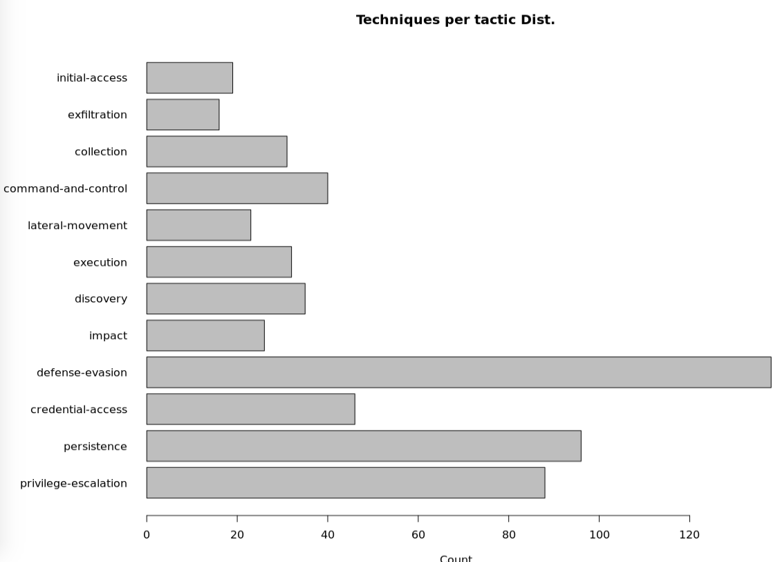
First let’s look at a distribution (number) of Techniques (INCLUDING sub-techniques) associated to each Tactic in the Matrix:
And next the “usual” (for me) network graph. In that case, it might come in handy (in a future) to look at the “centrality” of techniques, maybe showing their relative importance, and/or pivotal role in a Kill-Chain. So a quick & dirty visualization (in blue, the Tactics, in red, the Techniques):
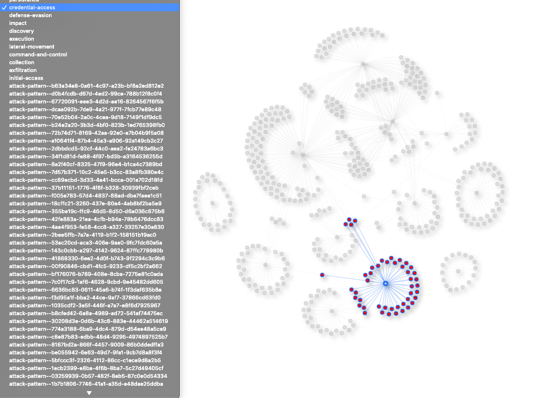
Think of it as a draft graph. But you could add context, filters, and set up a Shiny Dashboard to look at such data.
As a first thing anyway, it stands out that some of the Tactics have “dedicated techniques”, thereby creating two distinctly isolated sub-graphs: “Impact” and “Exfiltration”.
You can also “travel” different paths through tactics using different Techniques, for example:
Collection to Credentials Access, from there to Defense Evasion and then to Lateral Movement, etc.
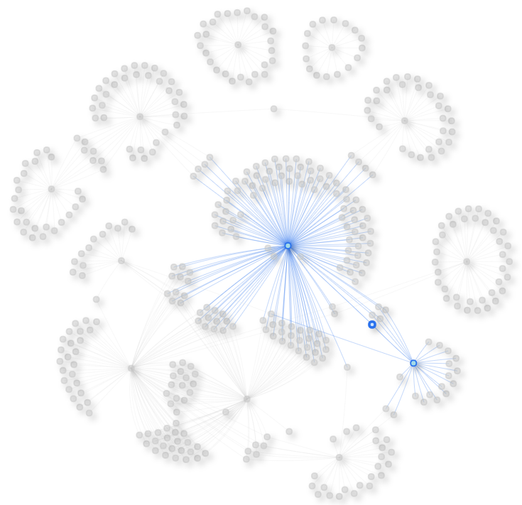 You can just follow the steps, and for each step, you could dive into the technique. That’s just one example usage, though.
Conclusions
There are libraries in R to read in Data in many formats, JSON – a common format – among them. It’s then easy (depending on how you go about it) to move to the more traditional data.frame or data.table format to be used for later analysis.
I’ve skipped lots of steps. For instance, there is much cleaning to be done on the dataset after import, but it was a bit beyond the point here.
Finally, having a look at MITRE ATT&CK is a great exercise. Looking at what is being done “out there” to attack, instead of always “looking at the inside data”, helps contextualize and – at the very least – gives a framework for a potential prioritization of detection needs.
Lots can be done analysing data of MITRE, SO MUCH more than just having a quick look like we did here, but I only have had little spare time these past few weeks, so I thought it was worth writing one quick post instead of going for a full-blown analysis.
Also, I will be creating a “Home Lab” so I might be a bit busy to write here in the next few weeks, but I’ll try to keep writing from time to time; I might just miss (again) the weekly-post mark I’ve set for myself. But the Lab might prove useful as a source of contents for future posts, who knows.
References
My code on my GitHub account for the above (not very optimized though)