Last week we set up the context for today’s entry.
Warning: Today’s post is possibly one of the most ambitious I have written in this Blog, in terms of “concepts touched”. It is very practical, and hopefully neither boring nor completely unintelligible.
More importantly: It’s about what everyone talks about, “Machine learning”. (It’s hence about what most mean to say when they say “Artificial Intelligence”, too.)
Let’s get to it.
Getting the data
First, we’ll need some data. Unfortunately I can’t seem to locate the reference from which I got the sample logs, but that won’t be an issue, as the goal is precisely to explain something that we want to make work with different log samples. (Also, whatever the source, I do know I made sure to only use legally, “open-data” logs…)For today’s purpose, let’s just assume we have:
- 100 lines of Apache logs
- 96 lines of BlueCoat logs
And let’s consider this “balanced enough”. This is NOT a lot of data (far from it), but that will be just about enough for today’s demo.
The pre-processing
Now a web server logs (for example) has several dynamic things to it. As an example: It might contain the originated IP that made the web request, or a URL requested, specific to a given virtual server.
Now we want to get rid of that. What we want is to generically recognise a “web server log”, not THIS web server logs. Otherwise, well, we couldn’t generalise (see last week’s notes).
OK, so we’ll get rid of some of the variability that is not SPECIFIC to one Web server. This is, as always, a simplified approach, for “educational purposes” mostly. Then we’ll read our sample data:
# A simple cleaning function for web-related logs:
clean_noisy_values <- function(tempdf) {
 # Remove IP addresses:
 tempdf$Log <- gsub("[0-9]{1,3}\\.[0-9]{1,3}\\.[0-9]{1,3}\\.[0-9]{1,3}",
  " ", tempdf$Log)
 # Remove DateTime
 #2005-04-05 18:36:57
 tempdf$Log <- gsub("[0-9]{4}\\-[0-9]{2}\\-[0-9]{2} [0-9]{2}\\:[0-9]{2}\\:[0-9]{2}",
  " ", tempdf$Log)
 #09/Mar/2004:22:36:21
 tempdf$Log <- gsub("[0-9]{2}\\/[A-Za-z]{3}\\/[0-9]{4}\\:[0-9]{2}\\:[0-9]{2}\\:[0-9]{2}",
  " ", tempdf$Log)
 # finally, remove URLs
 tempdf$Log <- gsub("([A-Za-z0-9-]+\\.)?[A-Za-z0-9-]+\\.[a-z]{2,3}",
  "URIComponent", tempdf$Log)
 return(tempdf)
}

# Load sample Apache logs
mydf <- data.frame(readLines(con="/mnt/R/data/sample_apache.log"))
names(mydf) <- c("Log")
mydf$class <- "apache"

#Load sample BC logs
mydf2 <- data.frame(readLines(con="/mnt/R/data/sample_bc.log"))
names(mydf2) <- c("Log")
mydf2$class <- "Bluecoat"
mydf2 <- mydf2[-seq(1:4),]

mydf <- clean_noisy_values(mydf)
mydf2 <- clean_noisy_values(mydf2)

mydf <- rbind(mydf, mydf2)
rm(mydf2)

# Quick check:
mydf[1,]
mydf[101,]
## Fair enough. We now have 1 dataset with 100 apache logs, and 96 BC Logs.
# All "somewhat cleaned"
Please bear in mind, this is a demo meant towards explaining a concept. So be gentle. (It will soon turn out that the whole exercise is mostly moot, but the concept and code approach are valid ;))
Codifying the information
Now what we have is, in essence, text.
Let’s see if there is something in the “Natural Language Processing” (a.k.a. “NLP”) toolbox to help us prepare our data for our ML algorithms to use.
We will use the TF-IDM approach. This basically counts words in documents and helps separate words that appear in some of the documents, but not the others. Allow me to skip on the details, just remember this: “Terms Frequency, Inverse-Document Frequency”. This is a very commonly used tool to work with, in documents classification).
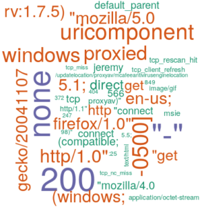
### Section 2 ###
# So here we'll create a Terms Documents Matrix
# The idea is to represent words in terms of frecuencies, per "line"/Document
## Now let's do some basic NLP

library(tm) # for Corpus
library(SnowballC)
library(wordcloud)

review_corpus <- Corpus(VectorSource(mydf$Log))
review_corpus <- tm_map(review_corpus, content_transformer(tolower))
## There are more options, but we will NOT use them here.
# review_corpus <- tm_map(review_corpus, removePunctuation)
# review_corpus <- tm_map(review_corpus, stripWhitespace)

#Let's have a look:
inspect(review_corpus[1])
inspect(review_corpus[101])

## OK so now we will work with the presence, or not, of words in a line:
review_dtm <- DocumentTermMatrix(review_corpus)
review_dtm
inspect(review_dtm[98:102, 1:5])
# How many distinct "words" do we have?
dim(review_dtm)

# remove sparse terms. These are rarely present:
review_dtm <- removeSparseTerms(review_dtm, 0.99)
review_dtm
inspect(review_dtm[1,1:20])
inspect(review_dtm[101,1:5])
# After the first cleaning up:
dim(review_dtm)
# With our sample dataset, we're down to "only" 152 terms...

# What are the most frequent terms in each subset?
findFreqTerms(review_dtm[1:100,], 10)
findFreqTerms(review_dtm[101:196,], 10)
# "\"mozilla/4.0" appears in both in our example, for instance...

# Let's plot the resulting terms frequencies matrix for all entries:
freq <- data.frame(sort(colSums(as.matrix(review_dtm)), decreasing=TRUE))
# barplot(freq[,1], ylab = rownames(freq), horiz = TRUE)
wordcloud(rownames(freq), freq[,1], max.words=50, colors=brewer.pal(1, "Dark2"))
# Not very interesting in and of itself. However, do notice the "word": -0500]
For now we’ve gotten around the Terms Frequencies.
### Section 3 ###
# Another concept is the representation of one word compared to the number of
# documents it appears in. A word can be unfrequent in one document, but
# very common across documents, for example. Or the contrary.
# Let's assign a value for that:

# tf-idf: terms Frecuency vs inverse-document-frecuency
review_dtm_tfidf <- DocumentTermMatrix(review_corpus, control = list(weighting = weightTfIdf))
review_dtm_tfidf <- removeSparseTerms(review_dtm_tfidf, 0.95)
review_dtm_tfidf
inspect(review_dtm_tfidf[1,1:5])
inspect(review_dtm_tfidf[101,1:5])

# We could have a look at that now:
#freq <- data.frame(sort(colSums(as.matrix(review_dtm_tfidf)), decreasing=TRUE))
#wordcloud(rownames(freq), freq[,1], max.words=100, colors=brewer.pal(1, "Dark2"))


# OK we still have the original log and the class for each entry.
# Let's create a "reviews" object with the class and the tf-idf matrix
mytfidf <- as.matrix(review_dtm_tfidf)
reviews <- cbind(mydf$class, mytfidf)
reviewsdf <- as.data.frame(reviews)

head(reviews[,1:5])
tail(reviews[,1:5])

# Now do you think the computer will be able to distinguish between the two
# classes of logs?
## Remember, the line number corresponds to Apache (1-100) and BC (101-196)
# But before, could WE?
# Visualize difference between terms distributions:
heatmap(mytfidf)
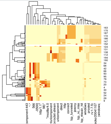
If you have followed a bit the code so far, you’ll see that our logs are, technically, separated sequentially in our dataset. So the first rows are all of the type Apache, while all the last rows are Bluecoat. Visually, a HeatMap of the TF-IDF already clearly shows that the “words” in one category and those in the other are just about as separated as it gets (this is good news, it means our future classifier(s) should have it easy).
Fair enough.
Actually Doing Supervised Learning!
Today, we’ll demo three rather common Machine Learning Algorithms: RPART (also known as “partitioning trees”), SVM (Support Vector Machine) and simple Neural Networks.
Thanks to R libraries, we do not have to worry about how each actually works. This is not to say we shouldn’t care, and I definitely recommend brushing-up on the concepts. But as today’s objective is to be very practical, I’ll allow myself to skip the concepts (incidentally, it’s not THAT easy to summarise each in a text format in only one “blog entry”, at least unless I want you, my dear reader, to disconnect).
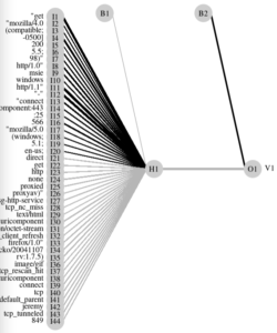
### Section 4: ###
# Can we train a PC to "automagically" distinguish between the two classes?
# Also, can we do it WITHOUT telling it any preset "rule".
# Bear in mind this:
# In theory, our goal is to be able to pass our PC two sets of logs of two
# different sources for training. Any two different sources.
# After which, we would ask our laptop to train on that, and create a
# classifier to distinguish between the two types.
# Again, WHICHEVER two different log types.
# Or twitter users, or books authors... That's why this is important.
# We don't tell the script anything about the content.
# Up to a point, we would not need to even look at it...

# Let's separate train & test - 1 fold, 70%
id_train <- sample(nrow(reviews),nrow(reviews)*0.7)
reviewsdf.train <- reviewsdf[id_train,]
reviewsdf.test <- reviewsdf[-id_train,]

library(rpart)
library(rpart.plot)
library(e1071)
library(nnet)


# Required for SVM & NNet:
reviewsdf.train$V1 <- ifelse(reviewsdf.train$V1 == "apache", 0, 1)
reviewsdf.test$V1 <- ifelse(reviewsdf.test$V1 == "apache", 0, 1)
reviewsdf.train[] <- lapply(reviewsdf.train, as.numeric)
reviewsdf.test[] <- lapply(reviewsdf.test, as.numeric)
# Train Partitioning Tree
reviewsdf.tree <- rpart(V1~., method = "class", data = reviewsdf.train);
prp(reviewsdf.tree)

Nice. Our first algorithm (rpart) is an open book about the feature it has chosen. Moreover, it’s almost not even a “tree”, it’s a simple “if”: either the document contains a certain frequency of the term “-500]”, or it doesn’t. At least, based on our training data. And that’s a good predictor (a great one). Which is why I said at the beginning, this particular example turns out to be a bit moot. Nevertheless, we’ll keep going, as the concepts still stand as-is.
What does it look like when we test it, against the Test data subset?
In a Contingency Table (another importante concept, which quickly gives us information about how well our model classifies stuff in the right class):

That is, everything in the test data subset has been correctly classified (Predicted) compared to what we actually know about the data (Observed). A great classifier for this use-case. The same exercise for a MUCH BIGGER sample of data for each class, could possibly work just as well. And we would essentially be done!
Next time we receive a sample of logs that can either be Apache or Bluecoat (well, nuanced: with similar logging format, which hopefully would be standardized across an organization), we can just pass it to our RPART model, and it will tell us whether the sample comes from an Apache or Bluecoat Proxy.
Let’s keep going nevertheless. What about other algorithms, sometimes considered more “robust”?
Testing the use of SVM and NeuralNet
This is now more “for show”, but let’s suppose our RPART model for some reason misbehaves with more real-life data. So we decide (in that scenario) to test and see if other algorithms could work better.
Well, in R, with the data already in the right format, it CAN be quite easy:
# Train SVM
reviewsdf.svm <- svm(V1~., data = reviewsdf.train);
# Testing SVM
pred.svm <- predict(reviewsdf.svm, reviewsdf.test)
table(reviewsdf.test$V1,round(pred.svm),dnn=c("Obs","Pred"))
There. Suffice to say, SVM behave just as good as our Partitionning Tree above.
What about a simple Neural Network (sooo fashionable, along with all the “AI” hype)? Well:
# Train NNet
reviewsdf.nnet <- nnet(V1~., data=reviewsdf.train, size=1, maxit=500)
# Testing NNet
prob.nnet <- predict(reviewsdf.nnet,reviewsdf.test)
pred.nnet <- as.numeric(prob.nnet > 0.5)
table(reviewsdf.test$V1, pred.nnet, dnn=c("Obs","Pred"))
And we get to the same result.
Remember that based on our sample data, there is a “feature” that on its own is able to bear all the prediction power with perfect accuracy. But in the real world, you might have to work a bit harder, even beyond choosing between 2, 3 or more algorithms.
In the real world, you will probably have to deal with “hyper-parameters” for some of the algorithms. This is beyond today’s goals. But suffice to say, for example, that a Neural network can have one OR several layers, each with a number of neurons, and can use different activation functions, that will play nicely or not depending on the data…
Which is why it is a good idea to test several algorithms and configurations. Some algorithms will be generally better suited for some specific use cases (e.g. CNNs are known to work nicely for image classification, like our “cat vs dog” example from last week).
In other words: This example has been very gentle on us. It might not always be that easy. I point this out because I don’t want to mislead anyone about how “magical” things are here 🙂
Reducing Features/Dimensions
OK, let me go into one last concept for today, so that I know I have covered a good part of “the basis” that one should consider when talking about Machine Learning Algorithms.
Once again, I’ll go practical: I’ll use the Principal Component Analysis (a.k.a. “PCA”) on my cleaned TF-IDF dataset generated earlier.
The goal is to see if we can create a classifier that doesn’t necessarily use ALL the terms in our cleaned dataset and still get to an acceptable classification power. More precisely though, we want to see if we can use less pre-calculated “components”, derived from our original variables (the words), than the original variables.
Very very simplified: PCA uses Vectors and orthogonality to “project” two or more dimensions onto, well, less dimensions. It’s a bit mathematical. But they it just GREAT in this YouTube video by “StatQuest” (one of the best explanations out there, if you ask me, on this particular topic):
Whatever the mathematical background, our goal is to see if we can use LESS parameters to train (and test) our models, so that they are made (possibly much) more efficient. This can be important in a real-world-production data-product, for example one made to analyse millions of variables (if not transformed). And MAYBE a controlled trade-off in accuracy is acceptable. That all depends on the objectives/context/environment.
On with it.
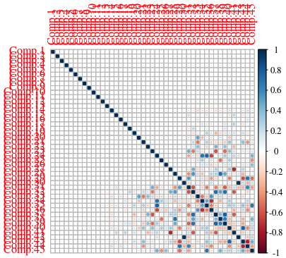
For now, we have 45 dimensions (with our dataset, that is). Let’s pass that through our PCA algorithm. What we aim for is for AS LITTLE CORRELATION as possible between the different components.
# ...
pcatrain <- princomp(as.matrix(reviewspca.train2), cor=TRUE, scores = TRUE)
pcatest <- princomp(as.matrix(reviewspca.test2), cor=TRUE, scores = TRUE)
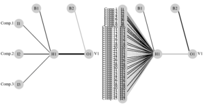
In a CorrPlot like the following one, the first few components are clearly NOT correlated, which is what we want, as each component BRINGS INFORMATION to help with the classification. The more two components are correlated, the less having both of them in the dataset brings value for our classifier.
This is turning quite nicely. Let’s have a visual look of “how much classification power” (information, in this case variance) is explained by the top 10 newly created features (“components”):
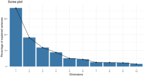
The above graph indicates that we might be able to put about 67% of the variance in the data with only 3 components (versus the 45 original variables!). 67% is not great, but you get the point: With the 6 first components, we get a reasonable total, to almost 85%).
Let’s put this idea to the test
I will repeat the above trainings and testings of our NeuralNet, but with 3 and 30 components, respectively, and just summarise the resulting classification errors. It’s pretty clear that IF our Neural network is able to correctly classify our datasets with less “neurons”, it will be simpler, less “computationally expensive”, probably much faster…
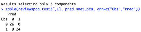
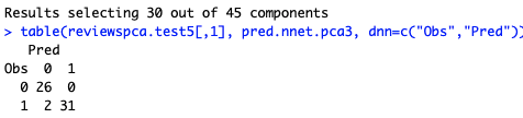
Maybe 3 dimensions was too much simplifying. But with 66% of the amount of original variables, we are able to get about 97% accuracy (57/59 correctly classified logs!).
Conclusions
We’re done!
I know this has been long, and complex.
Hopefully, along with last week’s post, you have gotten some conceptual understanding of Supervised Machine Learning concepts. You’ve also seen that it is possibly NOT that hard to implement, even when applied to a specific, real-world use-case (believe you me, it is a real world necessity (albeit very specific) to be able to distinguish log-source types, the more automatically, the better).
Hopefully, you’ll have taken back something (if you’re new to the subject) and have now an idea of why Machine Learning could actually be a great tool to help us in our daily work.
That is, if it is used correctly, and put to use in sensible use-cases.