Intro
First, let me say, I know, it’s been a while. And that’s alright. I have plenty of good excuses 🙂 Now that doesn’t mean I should completely forget about this my little Blog.
OK, so, for today: I’ve been studying Operations Research for about 3 months now, and we’re getting (in the Master course) to simulation as a means to do optimization (I guess, for what some call “simheuristics”). OK, and what’s cool, is I get to do some exercises, and as the exercises are never proposed in R, I get to do what I want here to reproduce some of it.
So, today, Monte-Carlo.
The context
In the past, I’ve prepared a small simulation that would potentially help “frame” the operations of a SOC, and its analysts, team sizing, etc. I wrote about that here and here. Already back then, I mentioned “Alerts are not received at a set interval” (well, not a fixed one, anyway). Instead, we might consider the alerts are generated following some other density function/probability distribution.
The most common distributions for input calls rates to a datacenter are probably Poisson, Exponential, or Weibull (or even Beta…), and in any case, it doesn’t hurt to have some level of familiarity with a few distributions (on top of the above, I’d say… The Normal, lognormal, triangular, a maybe a few others).
More context
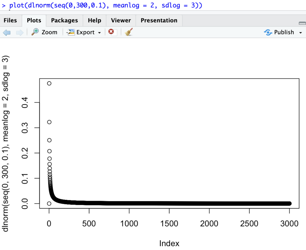
OK, so “simply” generating data from a certain density function is not all that hard in R. Just call one of stats package functions for it, say a LogNormal density function:

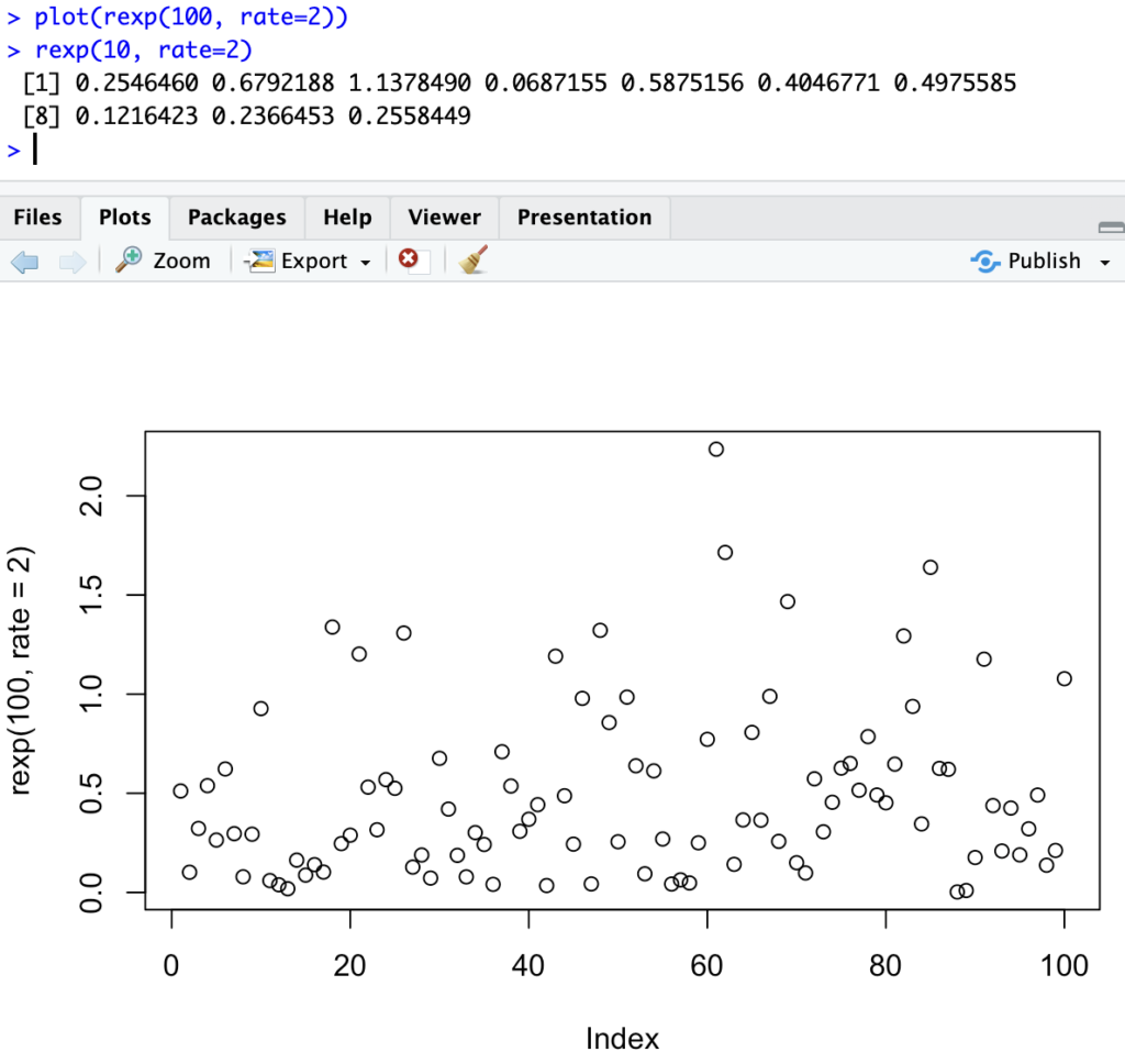
You can also generate sample data from such a distribution, from say an Exponential distribution:

The tweak though is to decide, from a set of data points (observations), which of such distributions would best fit. Here the goal is to find a valid theoretical distribution that “fits” our observations (today, univariate), so that we can then use that theoretical distribution to generate as many sample input values to our system. Each such distribution has parameters, though, so not only do we need to know whether to use an exponential or a beta, but also, with which parameters should those best “fit” our observations.
So supposing our alerts are reaching our SIEM at a rate (say, alerts per hour?) that can be akin’ to a Poisson distribution, what are the parameters of such a Poisson distribution?
Even better, which is it in the first place, a Poisson distribution or an Exponential? Finding that out (“fitting” a distribution) will enable us to simulate various executions of our system (say, our SOC simulator) with representative input (alerts reception rate), which is what Monte Carlo is all about.
That would greatly improve the validity of our toy simulator. After all, as many say (I’ve invented NOTHING in this blog post… Just applying/learning): What’s worse, exact answers to an incorrect simulation model, or approximate answers to the right simulation?
Interlude
While working on the code (coming next), I kept looking at the homework I was given, and there I came across a paper, that, simply put, I think is marvellous:
INTRODUCTION TO MONTE CARLO SIMULATION
If at all interested in the subject, and not yet quite clear what Monte-Carlo is all about, please oh please, give this short paper a chance. You’ll thank me later.
Back to work: Basic fitting, visually
Time to do some actual R programming. Let’s use classics here for now. The MASS package comes with the VERY handy “fitdistr()” function. I know (because I looked it up!) there are other more advanced packages out there that help with this very task (fitting a density function to some data), but sometimes I need to get a better feeling of what’s happening doing things, so here we are programming our own function…
Here the function (as formatting is not great, I’ll just post the sample code on my Github account).
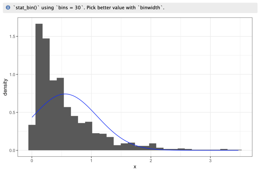
This short sample function should generate some Plot output with a histogram of our “real” data (which we can then generate to test fitting or not, visually), and a density function (blue line) for the fitted (parameterized) function that we have selected.
We can then test it with some datasets that we “know” ahead of the fitting will fit one of the distributions (even when a little noise is added)…
noise <- runif(1000,0,1) # to make it a bit harder for the fitting estimations...
my_normvec <- rnorm(1000, mean=3, sd=2) + noise # self describing
my_expvec <- rexp(1000, rate=2) + noise/10 # Generating 1000 numbers of exponential with lambda 2
my_lognormvec <- rlnorm(100, meanlog=1, sdlog=2) + noise*5

vis_compare_hist(my_normvec, "normal") # Good apparent fit
vis_compare_hist(my_normvec, "exponential") # must have positive values only! That's why we use tryCatch.
vis_compare_hist(my_expvec, "exponential") # Good apparent fit
vis_compare_hist(my_expvec, "normal") # clearly not matching...
vis_compare_hist(my_lognormvec, "lognormal") # ...
For which on of the outputs (that of the Exponential) is:

Whereas we can see, trying to “fit” a normal distribution to an exponential-based dataset, isn’t as good a fit, visually:

And as a final note for today (this is part 1 of maybe 2 or 3 entries…), we can generate data from a fitted function to a given dataset with “just” three lines (provided, for now, we know upfront which distribution we’re expecting, and are only looking for its parameters…)
# Future use: One can generate random samples from a fitted distribution, to feed a simulation for instance...:
t_fit <- fitdistr(my_normvec, "normal") # fitting a distribution to some data
t_fit$estimate # looking at the estimated parameters for the fitted function
sample_fit <- rnorm(t_fit$n, t_fit$estimate) # generating n values with the "fitted" distribution parameters
Conclusions
Now IF you have opened (and then checked more thoroughly) the paper recommended above, you might have found that the graphs proposed above look somewhat similar to doing a Chi Square Test. As they put it in the referenced paper (really, have a look):
“The Chi-square test can be thought of as a formal comparison of a histogram of the data with the density or mass function of the fitted distribution.”
Now if that’s not what we’ve done visually today…
There will be more entries on the topic, but I’m still quite busy these days with homework on top of real daily work… So it will come when it will come.
A thing to be tested is the fitdistrplus package and its possibilities, for instance. We’ll have to wait and see…
Resources