Intro

Continuing with this simple “series” (see here and here), I implement the next algorithm proposed by the reference book, but in R.

This time around, it’s the turn of “Simulated Annealing”.

Nice parallel

I like how the concept of molecules excitement and temperatures is used for this algorithm. All in all, it’s a bit different from Gradient Descent in that it allows to keep going with WORSE results in some cases, proportional to the progress, so that it explores better the overall range of possible values. This is supposed to ensure that this algorithm will in fact avoid falling in local minimum, and so this is better for situations where there are multiple minima.

That said, here the code for this algorithm. I haven’t made any effort to make this implementation “good” or fast, mind you, but it’s valid for a bi-variate function.

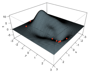
And here the results. This was not surprising after the algorithm was understood, but still, one can tell it was off-track in this example iteration, and still got to the right results in the end.

Conclusions

At this point, we might want to look into optimization that work also for non-differentiable functions (maybe). That’s a probable future post 🙂