Intro
I have some more spare time for the upcoming few weeks, and I haven’t had the opportunity to take the “Metaheuristics” course in the Master, and so I feel I’m missing out a bit… But then, what precludes me from learning on my own?
So I came across a book (I spend a bit too much time in book stores just “browsing”… Or buying books online) about “Optimisation” in Matlab. As it turns out, this appears to be in fact a great book to understand a few algorithms of the field of “Metaheuristics”.
First thing First
Before I start with optimization per-se, as the books relies somewhat heavily on two visualizations, Contours and 3D perspectives of bi-variate functions, I have to get acquainted with the necessary R code for just that.
The code for that is all in here.
Aside from learning that the base graphics in R are very capable, with “contour()” and “persp()” readily available, I’ve had to learn what Azimuth meant… Thankfully given the context, it wasn’t hard, and the Wikipedia is always helpful.
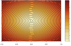
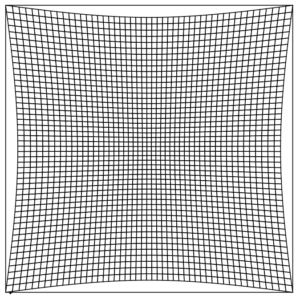
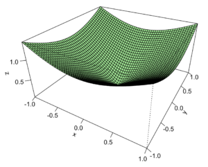
Here the results for today. I generate a 3D cone, and then we visualize through a couple of drawings that will be helpful later on.
A contour plot will show altitudes in 2D, which can be helpful when visualizing say “where is the minimum altitude”:

A Contour Plot
Then the 3D perspective visualization can be as bad as this:

Or a bit nicer, like so:

Next time
In the next blog entry, I will be discussing one of the first algorithms the book comments: Gradient Descent.