Intro
I finally passed the last semester of the Master degree I’m taking (slowly, but with much pleasure).
One of the last things I learned was about a practical application of Eigenvalues, in context of Spectral Decomposition of Adjacency Matrices… Big words all of them, but let’s just say it’s a valuable thing for studying graphs, and as we know graphs have many applications to represent things (systems, social setups, etc.).
Summary
In short, we can compare 2 graphs and decide which one of them is most near to being bipartite, using a “simple” calculation.
It wasn’t simple to me, I had to brush up once again about what Eigenvalues, Eigenvectors and (new to me completely) spectral analysis was all about and (most important to me) how to get to those things and WHY.
Shortening the post
Although I’ve learned a (slightly and anyway equivalent) different equation for the Bipartivity Index:

As it turns out, after understanding it all on my own, while researching for this post, I came across a paper that details the step-by-step of it all, and so I shall not re-write it all here to no added value, please check the first reference below.
A bit of R code
In R, it’s pretty easy to get “directly” to the Eigenvalues of a given matrix (as long as the set of them exists, that is…), by running this:
> print("For Bipartite Graph:")
> m_bip <- matrix(c(0,0,1,1,1,1,1,1, 0,0,1,1,1,1,1,1, 1,1,0,0,0,0,0,0, 1,1,0,0,0,0,0,0,
      1,1,0,0,0,0,0,0, 1,1,0,0,0,0,0,0, 1,1,0,0,0,0,0,0, 1,1,0,0,0,0,0,0),
      nrow=8, byrow = TRUE)
> ev <- eigen(m_bip)
> round(ev$values, 10)  # Rounding to "see" what it actually should be, many 0's

[1] 3.464102 0.000000 0.000000 0.000000 0.000000 0.000000 0.000000 -3.464102
But doing the math and understanding the steps behind it is more interesting (at least once in a lifetime), to get a sense of understanding. So here we can use a different approach (not fast) to get to the “characteristic polynomial” of a matrix, with the following steps:
library(Ryacas)
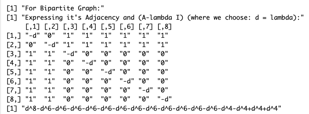
m_bip <- matrix(c("-d",0,1,1,1,1,1,1, 0,"-d",1,1,1,1,1,1, 1,1,"-d",0,0,0,0,0, 1,1,0,"-d",0,0,0,0, 1,1,0,0,
"-d",0,0,0, 1,1,0,0,0,"-d",0,0, 1,1,0,0,0,0,"-d",0, 1,1,0,0,0,0,0,"-d"),
nrow=8, byrow = TRUE)
print("Expressing it's Adjacency and (A-lambda I) (where we choose: d = lambda):")
print(m_bip)
yac_assign(ysym(m_bip), "M2")
yac_str("Determinant(M2)")
Which gives the following output:
And factorising the results will give us the set of eigenvalues to then feed into our index calculation:

Which leads to the same “Spectrum” (set of eigenvalues):

As we gave in fact as input a perfect bi-partite simple graph, the bipartivity index is maximum, e.g. 1:
> sum(cosh(ev$values)) / sum(exp(ev$values))

[1] 1
Conclusions
Once again here, I haven’t discovered the wheel… Well I never do, I guess.
But I came across this example application of the concept of Eigenvalues, and I liked it, and I was able to reproduce the steps using R code (unnecessarily complex in this instance just to make sure I understood the steps…).
That’s I guess an example of what I call “kaizen” and “deliberate practice”: Actually implementing something the hard way, not because I need to, but rather to understand how things work…
And it’s also thanks to studying the master and the Graph theory course that I came across this application.
I might never need any of this… But I like to think I understand a bit better now the potential value of “Eigenvalues”, and that’s enough of a reward for me.